将分tf2.0与tf1.0两大章节,分别重现TensorFlow教程中的关键章节。

8062097330.png
8062097330.png

TensorFlow2.0复习

keras机器学习基本知识

图像分类

该教程训练一个神经网络用于对衣物图像进行分类,如将鞋与衬衫分开。该教程使用tf.keras包,它是TF上构建和训练模型的高级API.

import tensorflow as tf
from tensorflow import keras

import numpy as np
import matplotlib.pyplot as plt
print(tf.__version__)
2.0.0

导入MNIST流行数据集

fashion_mnist = keras.datasets.fashion_mnist
(train_images, train_labels), (test_images, test_labels) = fashion_mnist.load_data()

载入这个数据集后,会得到4个Ndarray:

  • train_imagestrain_labels数组是训练集 -- 即模型用于学习的数据
  • 使用test_imagestest_labels测试集测试模型。

图像是28x28的ndarray,每一个像素的范围都是0,255。标签是一个整形数组,范围为0到9,与图像表征的衣服类型一一对应。

每一幅图像被映射到单个标签上。由于类名不包含于数据集,我们先把类名列出来以待后续使用。

class_names = ['T-shirt/top', 'Trouser', 'Pullover', 'Dress', 'Coat',
               'Sandal', 'Shirt', 'Sneaker', 'Bag', 'Ankle boot']

探索数据

训练模型前我们先检查下数据集的格式。以下结果说明训练集中共0.6billion张图片,每幅图片由28*28个像素组成:

train_images.shape
(60000, 28, 28)
# 训练集中有60000个标签
len(train_labels)
60000
# 每个标签都是0到9之间的整数
train_labels
array([9, 0, 0, ..., 3, 0, 5], dtype=uint8)
# 测试集中有10000张图片,每一幅图也是28*28像素
test_images.shape
(10000, 28, 28)
# 测试集包含10000个标签
len(test_labels)
10000

数据预处理

在将数据送入网络前,必须对其进行预处理。如果你查看训练集中的第一幅图片,你会发现像素值在0到255之间:

plt.figure()
plt.imshow(train_images[0])
plt.colorbar()
plt.grid(False)
plt.show()

在将值送入神经网络模型前,有必要将他们缩放到0到1之间。为了做这个操作,直接将值除255即可。训练和测试集必须以同种方式处理:

train_images = train_images / 255.0
test_images = test_images / 255.0

为了验证数据是正确格式,且你已经准备好训练和构建网络,我们绘制前43幅图片,并在图片下方显示其类名:

plt.figure(figsize=(10,10))
for i in range(43):
    plt.subplot(9,5,i+1)
    plt.xticks([])
    plt.yticks([])
    plt.grid(False)
    plt.imshow(train_images[i], cmap = plt.cm.binary)
    plt.xlabel(class_names[train_labels[i]])
plt.show()

构建模型

构建神经网络模型需要我们配置网络层,然后编译模型。

设置网络层

神经网络的基本构建单元叫做层。层根据输入数据抽取表征。这些表征对解决手头的问题一般很有意义。

大部分深度学习网络包含级联在一起的简单层。大部分层,例如tf.keras.layers.Dense都包含训练过程中学习的参数。

model = keras.Sequential([
    keras.layers.Flatten(input_shape=(28,28)),
    keras.layers.Dense(128, activation='relu'),
    keras.layers.Dense(10)
])

网络中的第一层,tf.keras.layers.Flatten将图片格式从2维数组转化为1维数组(784个像素)。可以想象它是拆分开像素的各行,再将它们连接起来。这一层没什么特别的参数要学习,它只是重新格式化数据。 在像素被压平之后,网络随即连接两个tf.keras.layers.Dense层。这些是紧密连接(或者称作全连接)的神经网络层。第一个Dense层有128个节点或者神经元。第二个(输出层)返回一个长度维10的序列,每个值都表示当前图片属于该类别的概率。

编译模型

在模型可以训练之前,还需要对它进行一些设置。这些设置是在compile步骤完成的:

  • 损失函数 - 这个函数衡量模型在训练过程中有多么精确。你的目标是最小化这个函数以使模型朝正确的方向优化。
  • 优化器 - 这表示模型如何根据它看到的数据和损失函数去更新参数
  • 评估指标 - 用于监控训练和测试步骤,以下的例子用准确率作为指标,即被正确分类的图片占全部图片的比例。
model.compile(optimizer='adam',
             loss=tf.keras.losses.SparseCategoricalCrossentropy(from_logits=True),
             metrics=['accuracy'])

训练模型

训练神经网络模型需要以下几个步骤:

  1. 将训练数据喂给模型。在例子中,训练数据对应于train_imagestrain_labels两个数组;
  2. 模型学习关联图片和标签;
  3. 你要求模型对测试集进行预测 -- 在这个例子中,既是test_images这个数组;
  4. 验证预测值与test_labels序列的标签对应。 #### 提供数据 为开始训练,调用model.fit方法,叫fit的原因是它将模型适配到训练数据的分布上:
model.fit(train_images, train_labels, epochs=10)
Train on 60000 samples
Epoch 1/10
60000/60000 [==============================] - 6s 105us/sample - loss: 2.4907 - accuracy: 0.7033
Epoch 2/10
60000/60000 [==============================] - 4s 67us/sample - loss: 0.6701 - accuracy: 0.7666
Epoch 3/10
60000/60000 [==============================] - 4s 68us/sample - loss: 0.5754 - accuracy: 0.8036
Epoch 4/10
60000/60000 [==============================] - 4s 72us/sample - loss: 0.5379 - accuracy: 0.8192
Epoch 5/10
60000/60000 [==============================] - ETA: 0s - loss: 0.5175 - accuracy: 0.82 - 4s 67us/sample - loss: 0.5178 - accuracy: 0.8288
Epoch 6/10
60000/60000 [==============================] - 4s 73us/sample - loss: 0.5025 - accuracy: 0.8339
Epoch 7/10
60000/60000 [==============================] - 4s 74us/sample - loss: 0.4878 - accuracy: 0.8375
Epoch 8/10
60000/60000 [==============================] - 4s 72us/sample - loss: 0.4842 - accuracy: 0.8405
Epoch 9/10
60000/60000 [==============================] - 4s 71us/sample - loss: 0.4791 - accuracy: 0.8441
Epoch 10/10
60000/60000 [==============================] - 4s 71us/sample - loss: 0.4747 - accuracy: 0.8437
<tensorflow.python.keras.callbacks.History at 0x2627486a5c8>

随着模型训练,损失和进度指标不断更新,模型最终在训练集达到了91%的精度。

评估精度

其后,我们对比一下模型在测试集上的表现:

test_loss, test_acc = model.evaluate(test_images, test_labels, verbose=2)
print('\nTest accuracy:', test_acc)
10000/1 - 1s - loss: 0.4512 - accuracy: 0.8165

Test accuracy: 0.8165

我们发现测试集上的精度要稍低于训练集上的精度。两个精度之间的差值说明出现了过拟合。在机器学习模型用于新的从未见过的输入时,它的表现变差,认为出现了过拟合。过拟合的模型记住了训练数据中的噪音和细节,以至于影响到模型在新数据上的效果。

预测结果

模型训练完后,我们可以用它来对一些新图片的类别进行预测。模型的原始输出向量称为对数logits。通过加入一个softmax层,可以将对数转化为概率分布,使结果更加便于理解。

probability_model = tf.keras.Sequential([model, tf.keras.layers.Softmax()])
predictions = probability_model.predict(test_images)
# 模型对所有测试集中的图片预测了类别,我们看看第一个预测的结果:
predictions[0]
array([3.95853505e-07, 5.04734352e-08, 4.52002773e-08, 1.04268434e-10,
       6.14671819e-07, 4.81123308e-04, 6.37260541e-07, 8.51320755e-03,
       1.08166132e-09, 9.91003871e-01], dtype=float32)

模型预测的类别是一个长度为10的数组。它们表征了模型给图片分属于10个类的“置信度”评价。可以用以下方式知道哪个标签有最大的置信度:

np.argmax(predictions[0])
9
# 所以模型认为图片最可能对应一个ankle boot靴子,或者class_names[9].
# 我们检查一下测试集标签,来证明模型的看法是对的:
test_labels[0]
9

绘制图片来看看所有的预测结果:

def plot_images(i, predictions_array, true_label, img):
    predictions_array, true_label, img = predictions_array, true_label[i], img[i]
    plt.grid(False)
    plt.xticks([])
    plt.yticks([])
    plt.imshow(img, cmap=plt.cm.binary)
    
    predicted_label = np.argmax(predictions_array)
    if predicted_label == true_label:
        color = 'blue'
    else:
        color = 'red'
    
    plt.xlabel("{} {:2.0f}%({})".format(class_names[predicted_label],
                                      100*np.max(predictions_array),
                                      class_names[true_label],
                                      color=color))
    
def plot_value_array(i, predictions_array, true_label):
    predictions_array, true_label = predictions_array, true_label[i]
    plt.grid(False)
    plt.xticks(range(10))
    plt.yticks([])
    thisplot = plt.bar(range(10), predictions_array, color='#777777')
    plt.ylim([0,1])
    predicted_label = np.argmax(predictions_array)
    
    thisplot[predicted_label].set_color('red')
    thisplot[true_label].set_color('blue')    

验证预测结果

模型训练完后,你可以用它进行预测。

我们先看看第1个图片,预测结果,以及对应的概率分布。正确的预测标签是蓝色的,不正确的是红色的。数值给出了预测标签的占比:

i = 0
plt.figure(figsize=(6,3))
plt.subplot(1,2,1)
plot_images(i, predictions[i], test_labels, test_images)
plt.subplot(1,2,2)
plot_value_array(i,predictions[i], test_labels)
plt.show()
i = 12
plt.figure(figsize=(6,3))
plt.subplot(1,2,1)
plot_images(i, predictions[i], test_labels, test_images)
plt.subplot(1,2,2)
plot_value_array(i,predictions[i], test_labels)
plt.show()

绘制一些图片和它们的预测结果就会发现,即便模型置信度很高,也可能是错误结果。

num_rows = 5
num_cols = 3
num_images = num_rows*num_cols
plt.figure(figsize=[2*2*num_cols, 2*num_rows])
for i in range(num_images):
    plt.subplot(num_rows, 2*num_cols, 2*i+1)
    plot_images(i, predictions[i], test_labels, test_images)
    plt.subplot(num_rows, 2*num_cols, 2*i+2)
    plot_value_array(i,predictions[i], test_labels)
    plt.tight_layout()
plt.show()

使用训练好的模型

我们终于可以用训练好的模型对单个图片进行分类了:

img = test_images[142]
plt.imshow(img)
<matplotlib.image.AxesImage at 0x2626cb6f908>

tf.keras模型已经经过优化,们可以对一个“batch”或者几何进行预测。所以即使你只是用单张图片,你也需要将它添加到列表中:

img = (np.expand_dims(img, 0))
print(img.shape)
(1, 28, 28)
# 现在对图片的正确标签进行预测:
predictions_single = probability_model.predict(img)
print(predictions_single)
[[8.6784530e-01 3.4884884e-04 1.2338771e-05 2.0001229e-02 4.8068767e-05
  4.6012540e-17 1.1174188e-01 2.8636104e-37 2.3276600e-06 5.6846246e-34]]
plot_value_array(1, predictions_single[0], test_labels)
_ = plt.xticks(range(10), class_names, rotation=30)
# keras.model.predict 返回一个二维数组,其中每个一维数组都对应
# batch中的一个图片。通过以下方式拿到我们对该批中唯一一幅图片的
# 预测结果:
np.argmax(predictions_single[0])
0

文本分类

使用 Keras 和 Tensorflow Hub 对电影评论进行文本分类

已有中文版本,此处仅列出代码。

from __future__ import \
absolute_import, division, \
print_function, unicode_literals

import numpy as np

import tensorflow as tf

import tensorflow_hub as hub
import tensorflow_datasets as tfds

print("Version: ", tf.__version__)
print("Eager mode: ", tf.executing_eagerly())
print("Hub version: ", hub.__version__)
print("GPU is", "available" if tf.config.experimental.list_physical_devices("GPU") else "NOT AVAILABLE")
Version:  2.0.0
Eager mode:  True
Hub version:  0.8.0
GPU is available
dir(tfds.Split.TRAIN)
['TEST',
 'TRAIN',
 'VALIDATION',
 '__add__',
 '__class__',
 '__contains__',
 '__delattr__',
 '__dict__',
 '__dir__',
 '__doc__',
 '__eq__',
 '__format__',
 '__ge__',
 '__getattribute__',
 '__getitem__',
 '__getnewargs__',
 '__gt__',
 '__hash__',
 '__init__',
 '__init_subclass__',
 '__iter__',
 '__le__',
 '__len__',
 '__lt__',
 '__mod__',
 '__module__',
 '__mul__',
 '__ne__',
 '__new__',
 '__reduce__',
 '__reduce_ex__',
 '__repr__',
 '__rmod__',
 '__rmul__',
 '__setattr__',
 '__sizeof__',
 '__str__',
 '__subclasshook__',
 '__weakref__',
 'capitalize',
 'casefold',
 'center',
 'count',
 'encode',
 'endswith',
 'expandtabs',
 'find',
 'format',
 'format_map',
 'index',
 'isalnum',
 'isalpha',
 'isascii',
 'isdecimal',
 'isdigit',
 'isidentifier',
 'islower',
 'isnumeric',
 'isprintable',
 'isspace',
 'istitle',
 'isupper',
 'join',
 'ljust',
 'lower',
 'lstrip',
 'maketrans',
 'partition',
 'replace',
 'rfind',
 'rindex',
 'rjust',
 'rpartition',
 'rsplit',
 'rstrip',
 'split',
 'splitlines',
 'startswith',
 'strip',
 'swapcase',
 'title',
 'translate',
 'upper',
 'zfill']
?tfds.Split.TRAIN.subsplit
Object `tfds.Split.TRAIN.subsplit` not found.
# 将训练集按照 6:4 的比例进行切割,从而最终我们将得到 15,000
# 个训练样本, 10,000 个验证样本以及 25,000 个测试样本

train_data, validation_data, test_data = tfds.load(
    name="imdb_reviews", 
    split=['train[:60%]', 'train[60%:]', tfds.Split.TEST],
    as_supervised=True)
Downloading and preparing dataset imdb_reviews/plain_text/1.0.0 (download: 80.23 MiB, generated: Unknown size, total: 80.23 MiB) to C:\Users\henryalps\tensorflow_datasets\imdb_reviews\plain_text\1.0.0...


Shuffling and writing examples to C:\Users\henryalps\tensorflow_datasets\imdb_reviews\plain_text\1.0.0.incompleteNJ9POX\imdb_reviews-train.tfrecord
Shuffling and writing examples to C:\Users\henryalps\tensorflow_datasets\imdb_reviews\plain_text\1.0.0.incompleteNJ9POX\imdb_reviews-test.tfrecord
Shuffling and writing examples to C:\Users\henryalps\tensorflow_datasets\imdb_reviews\plain_text\1.0.0.incompleteNJ9POX\imdb_reviews-unsupervised.tfrecord
Dataset imdb_reviews downloaded and prepared to C:\Users\henryalps\tensorflow_datasets\imdb_reviews\plain_text\1.0.0. Subsequent calls will reuse this data.
train_examples_batch, train_labels_batch = next(iter(train_data.batch(10)))
train_examples_batch
<tf.Tensor: id=200, shape=(10,), dtype=string, numpy=
array([b'This is a big step down after the surprisingly enjoyable original. This sequel isn\'t nearly as fun as part one, and it instead spends too much time on plot development. Tim Thomerson is still the best thing about this series, but his wisecracking is toned down in this entry. The performances are all adequate, but this time the script lets us down. The action is merely routine and the plot is only mildly interesting, so I need lots of silly laughs in order to stay entertained during a "Trancers" movie. Unfortunately, the laughs are few and far between, and so, this film is watchable at best.',
       b"Perhaps because I was so young, innocent and BRAINWASHED when I saw it, this movie was the cause of many sleepless nights for me. I haven't seen it since I was in seventh grade at a Presbyterian school, so I am not sure what effect it would have on me now. However, I will say that it left an impression on me... and most of my friends. It did serve its purpose, at least until we were old enough and knowledgeable enough to analyze and create our own opinions. I was particularly terrified of what the newly-converted post-rapture Christians had to endure when not receiving the mark of the beast. I don't want to spoil the movie for those who haven't seen it so I will not mention details of the scenes, but I can still picture them in my head... and it's been 19 years.",
       b'Hood of the Living Dead had a lot to live up to even before the opening credits began. First, any play on "...of the living dead" invokes His Holiness Mr. Romero and instantly sets up a high standard to which many movies cannot afford to aspire. And second, my movie-watching companion professed doubt that any urban horror film would surpass the seminal Leprechaun In the Hood. Skeptical, we settled in to watch. <br /><br />We were rewarded with a surprisingly sincere and good-hearted zombie film. Oh, certainly the budget is low, and of course the directors\' amateurs friends populate the cast, but Hood of the Living Dead loves zombie cinema. Cheap? Yeah. But when it\'s this cheap, you can clearly see where LOVE holds it together. <br /><br />Ricky works in a lab during the day and as a surrogate parent to his younger brother at night. He dreams of moving out of Oakland. Before this planned escape, however, his brother is shot to death in a drive-by. Ricky\'s keen scientific mind presents an option superior to CPR or 911: injections of his lab\'s experimental regenerative formula. Sadly, little bro wakes up in an ambulance as a bloodthirsty Oakland zombie! Chaos and mayhem! I think it\'s more economical to eat your enemies than take vengeance in a drive-by, but then again, I\'m a poor judge of the complexities of urban life. (How poor a judge? In response to a gory scene involving four men, I opined "Ah-ha! White t-shirts on everyone so the blood shows up. Economical! I used the same technique in my own low-budget horror film." Jordan replied, "No, that\'s gang dress. White t-shirts were banned from New Orleans bars for a time as a result." Oh.)<br /><br />A lot of the movie is set in someone\'s living room, so there\'s a great deal of hanging out and waiting for the zombies. But the characters are sympathetic and the movie is sincere-- it surpasses its budget in spirit. <br /><br />Zombie explanation: When man plays God, zombies arise! Or, perhaps: Follow FDA-approved testing rules before human experimentation! <br /><br />Contribution to the zombie canon: This is the first zombie movie I\'ve seen with a drive-by shooting. As far as the actual zombies go, infection is spread with a bite as usual, but quite unusually head shots don\'t work-- it\'s heart shots that kill. Zombies have pulses, the absence of which proves true death. And these zombies make pretty cool jaguar-growl noises. <br /><br />Gratuitous zombie movie in-joke: A mercenary named Romero. Groan. <br /><br />Favorite zombie: Jaguar-noise little brother zombie, of course!',
       b"For me this is a story that starts with some funny jokes regarding Franks fanatasies when he is travelling with a staircase and when he is sitting in business meetings... The problem is that when you have been watching this movie for an hour you will see the same fantasies/funny situations again and again and again. It is to predictable. It is more done as a TV story where you can go away and come back without missing anything.<br /><br />I like Felix Herngren as Frank but that is not enough even when it is a comedy it has to have more variations and some kind of message to it's audience....<br /><br />",
       b'This is not a bad movie. It follows the new conventions of modern horror, that is the movie within a movie, the well known actress running for her life in the first scene. This movie takes the old convention of a psycho killer on he loose, and manage to do something new, and interesting with it. It is also always nice to see Molly Ringwald back for the attack.<br /><br />So this might be an example of what the genre has become. Cut hits all the marks, and is actually scary in some parts. I liked it I gave it an eight.',
       b"I just finished a marathon of this series, and it became agonising to watch as it progressed. From the fictionalising of the historical elements, to O'Herlihy's awful accent in later episodes, the show just slumps the further it goes. If you are looking for some low quality production generalised WW2 fluff, then I could recommend season 1, but avoid anything after that, it degenerates into being one step from a soap opera, with increasingly worse story lines and sensibility.<br /><br />The old B&W film is by far the best of any form of entertainment with the Colditz name attached to it, and even that is not what one could hope for.",
       b'I am very sorry that this charming and whimsical film (which I first saw soon after it was first released in the early fifties) has had such a poor reception more recently. In my opinion it has been greatly underrated - but perhaps it appeals more to the European sense of humour than to (for example) the American: maybe we in Europe can understand and appreciate its subtleties and situations more, since we are closer to some of them in real life! Particular mention should be made of the limited but good music - especially the catchy and memorable song "It\'s a fine, fine night", which was issued separately on an HMV 78rpm record (10 inch plum label, I think!) in the fifties. I would urge anyone interested to give it a try if you get the chance: you may have a pleasant surprise.',
       b"Well i am going to go against the grain on this film so it seems. Being a self confessed horror fan I sat down to this not quite knowing what to expect. After 2 or 3 mins i actually found myself scared (quite rare). The film obviously has a small budget and is set around charing cross station but the films lack of money does not distract from the story. Yes the story is a bit far fetched and doesn't explain itself very well but THE CREEP is a class act and proceeds to slash and dismember anything that comes its way. MESSAGE FOR LADIES !!! THERE ARE CERTAIN PARTS OF THE FILM YOU SHOULD CLOSE YOUR EYES AT OR AT LEAST CROSS YOUR LEGS !! you will understand when you see it.<br /><br />All in all a good film and it makes a change to see a good slasher movie that actually scares",
       b'Even 15 years after the end of the Vietnam war "Jacknife" came not too late or was even superfluous. It\'s one of the few that try to deal with the second sad side of the war: The time after. Different from movies like "Taxi driver" or "Rambo" which use to present their main characters as broken heroes in a bad after war environment this movie allows the audience to face a different view on the Vietnam vets. Their development is shown very precisely before and especially after the war. The problems are obvious but in all this tragic there is always the feeling of some hope on the basis of love and friendship. "Jacknife" might be the quietest Vietnam movie ever but after almost 15 years this is really plausible and therefor justified. Moreover, it can make us believe that the war has not finished, yet; at least for some of us.<br /><br />The three main characters are amazing. De Niro has done one of his best jobs but Ed Harris is the star of this movie. Possibly,this was his best performance ever.',
       b'Before I explain the "Alias" comment let me say that "The Desert Trail" is bad even by the standards of westerns staring The Three Stooges. In fact it features Carmen Laroux as semi- bad girl Juanita, when you hear her Mexican accent you will immediately recognize her as Senorita Rita from the classic Stooge short "Saved by the Belle". <br /><br />In "The Desert Trail" John Wayne gets to play the Moe Howard character and Eddy Chandler gets to play Curly Howard. Like their Stooge counterparts a running gag throughout the 53- minute movie is Moe hitting Curly. Wayne\'s character, a skirt chasing bully, is not very endearing, but is supposed to be the good guy. <br /><br />Playing a traveling rodeo cowboy Wayne holds up the rodeo box office at gunpoint and takes the prize money he would have won if the attendance proceeds had been good-the other riders have to settle for 25 cents on the dollar (actually even less after Wayne robs the box office). No explanation is given for Wayne\'s ripping off the riders and still being considered the hero who gets the girl. <br /><br />Things get complicated at this point because the villain (Al Ferguson) and his sidekick Larry Fine (played by Paul Fix-who would go on to play Sheriff Micah on television\'s "The Rifleman") see Wayne rob the box office and then steal the remainder of the money and kill the rodeo manager. Moe and Curly get blamed. <br /><br />So Moe and Curly move to another town to get away from the law and they change their names to Smith and Jones. Who do they meet first but their old friend Larry, whose sister becomes the 2nd half love interest (Senorita Rita is left behind it the old town and makes no further appearances in the movie). <br /><br />Larry\'s sister is nicely played by a radiantly beautiful Mary Kornman (now grown up but in her younger days she was one of the original cast members of Hal Roach\'s "Our Gang" shorts). Kornman is the main reason to watch the mega-lame western and her scenes with Moe and Curly are much better than any others in the production, as if they used an entirely different crew to film them. <br /><br />Even for 1935 the action sequences in this thing are extremely weak and the technical film- making is staggeringly bad. The two main chase scenes end with stock footage wide shots of a rider falling from a horse. Both times the editor cuts to a shot of one of the characters rolling on the ground, but there is no horse in the frame, the film stock is completely different, and the character has on different clothes than the stunt rider. There is liberal use of stock footage in other places, none of it even remotely convincing. <br /><br />One thing to watch for is a scene midway into the movie where Moe and Curly get on their horses and ride away (to screen right) from a cabin as the posse is galloping toward the cabin from the left. The cameraman follows the two stooges with a slow pan right and then does a whip pan to the left to reveal the approaching posse. Outside of home movies I have never seen anything like this, not because it is looks stupid (which it does) but because a competent director would never stage a scene in this manner. They would film the two riders leaving and then reposition the camera and film the posse approaching as a separate action. Or if they were feeling creative they would stage the sequence so the camera shows the riders in the foreground and the posse approaching in the background. <br /><br />Then again, what do I know? I\'m only a child.'],
      dtype=object)>
train_labels_batch
<tf.Tensor: id=201, shape=(10,), dtype=int64, numpy=array([0, 0, 1, 0, 1, 0, 1, 1, 1, 0], dtype=int64)>
embedding = "https://tfhub.dev/google/tf2-preview/gnews-swivel-20dim/1"
hub_layer = hub.KerasLayer(embedding, input_shape=[], 
                           dtype=tf.string, trainable=True)
# 注意这里直接以函数形式调用hub_layer即可得到输出
hub_layer(train_examples_batch[:3])
<tf.Tensor: id=383, shape=(3, 20), dtype=float32, numpy=
array([[ 2.209591  , -2.7093675 ,  3.6802928 , -1.0291991 , -4.1671185 ,
        -2.4566064 , -2.2519937 , -0.36589956,  1.9485804 , -3.1104462 ,
        -2.4610963 ,  1.3139242 , -0.9161584 , -0.16625322, -3.723651  ,
         1.8498232 ,  3.499562  , -1.2373022 , -2.8403084 , -1.213074  ],
       [ 1.9055302 , -4.11395   ,  3.6038654 ,  0.28555924, -4.658998  ,
        -5.5433393 , -3.2735848 ,  1.9235417 ,  3.8461034 ,  1.5882455 ,
        -2.64167   ,  0.76057523, -0.14820506,  0.9115291 , -6.45758   ,
         2.3990374 ,  5.0985413 , -3.2776263 , -3.2652326 , -1.2345369 ],
       [ 3.6510668 , -4.7066135 ,  4.71003   , -1.7002777 , -3.7708545 ,
        -3.709126  , -4.222776  ,  1.946586  ,  6.1182513 , -2.7392752 ,
        -5.4384456 ,  2.7078724 , -2.1263676 , -0.7084146 , -5.893995  ,
         3.1602864 ,  3.8389287 , -3.318196  , -5.1542974 , -2.4051712 ]],
      dtype=float32)>
model = tf.keras.Sequential()
model.add(hub_layer)
model.add(tf.keras.layers.Dense(16, activation='relu'))
model.add(tf.keras.layers.Dense(1, activation='sigmoid'))

model.summary()
Model: "sequential"
_________________________________________________________________
Layer (type)                 Output Shape              Param #   
=================================================================
keras_layer (KerasLayer)     (None, 20)                400020    
_________________________________________________________________
dense (Dense)                (None, 16)                336       
_________________________________________________________________
dense_1 (Dense)              (None, 1)                 17        
=================================================================
Total params: 400,373
Trainable params: 400,373
Non-trainable params: 0
_________________________________________________________________
model.compile(optimizer='adam',
              loss='binary_crossentropy',
              metrics=['accuracy'])
history = model.fit(train_data.shuffle(10000).batch(512),
                    epochs=20,
                    validation_data=validation_data.batch(512),
                    verbose=1)
Epoch 1/20
30/30 [==============================] - 6s 198ms/step - loss: 0.7342 - accuracy: 0.5693 - val_loss: 0.0000e+00 - val_accuracy: 0.0000e+00
Epoch 2/20
30/30 [==============================] - 5s 150ms/step - loss: 0.6288 - accuracy: 0.6535 - val_loss: 0.6012 - val_accuracy: 0.6827
Epoch 3/20
30/30 [==============================] - 4s 147ms/step - loss: 0.5822 - accuracy: 0.7035 - val_loss: 0.5648 - val_accuracy: 0.7171
Epoch 4/20
30/30 [==============================] - 5s 151ms/step - loss: 0.5438 - accuracy: 0.7380 - val_loss: 0.5320 - val_accuracy: 0.7472
Epoch 5/20
30/30 [==============================] - 5s 151ms/step - loss: 0.5065 - accuracy: 0.7693 - val_loss: 0.5013 - val_accuracy: 0.7729
Epoch 6/20
30/30 [==============================] - 5s 151ms/step - loss: 0.4721 - accuracy: 0.7935 - val_loss: 0.4707 - val_accuracy: 0.7926
Epoch 7/20
30/30 [==============================] - 5s 151ms/step - loss: 0.4359 - accuracy: 0.8181 - val_loss: 0.4423 - val_accuracy: 0.8078
Epoch 8/20
30/30 [==============================] - 4s 150ms/step - loss: 0.3999 - accuracy: 0.8367 - val_loss: 0.4140 - val_accuracy: 0.8228
Epoch 9/20
30/30 [==============================] - 5s 150ms/step - loss: 0.3695 - accuracy: 0.8518 - val_loss: 0.3899 - val_accuracy: 0.8359
Epoch 10/20
30/30 [==============================] - 5s 150ms/step - loss: 0.3370 - accuracy: 0.8676 - val_loss: 0.3697 - val_accuracy: 0.8469
Epoch 11/20
30/30 [==============================] - 5s 155ms/step - loss: 0.3065 - accuracy: 0.8818 - val_loss: 0.3514 - val_accuracy: 0.8549
Epoch 12/20
30/30 [==============================] - 4s 147ms/step - loss: 0.2848 - accuracy: 0.8946 - val_loss: 0.3368 - val_accuracy: 0.8635
Epoch 13/20
30/30 [==============================] - 4s 148ms/step - loss: 0.2639 - accuracy: 0.9033 - val_loss: 0.3259 - val_accuracy: 0.8670
Epoch 14/20
30/30 [==============================] - 5s 151ms/step - loss: 0.2419 - accuracy: 0.9109 - val_loss: 0.3173 - val_accuracy: 0.8704
Epoch 15/20
30/30 [==============================] - 5s 151ms/step - loss: 0.2265 - accuracy: 0.9188 - val_loss: 0.3144 - val_accuracy: 0.8699
Epoch 16/20
30/30 [==============================] - 4s 148ms/step - loss: 0.2098 - accuracy: 0.9256 - val_loss: 0.3046 - val_accuracy: 0.8738
Epoch 17/20
30/30 [==============================] - 4s 147ms/step - loss: 0.1939 - accuracy: 0.9333 - val_loss: 0.3023 - val_accuracy: 0.8758
Epoch 18/20
30/30 [==============================] - 5s 150ms/step - loss: 0.1821 - accuracy: 0.9383 - val_loss: 0.2993 - val_accuracy: 0.8773
Epoch 19/20
30/30 [==============================] - 4s 147ms/step - loss: 0.1722 - accuracy: 0.9429 - val_loss: 0.2977 - val_accuracy: 0.8782
Epoch 20/20
30/30 [==============================] - 4s 150ms/step - loss: 0.1580 - accuracy: 0.9497 - val_loss: 0.2988 - val_accuracy: 0.8786
results = model.evaluate(test_data.batch(512), verbose=2)
for name, value in zip(model.metrics_names, results):
  print("%s: %.3f" % (name, value))
49/49 - 4s - loss: 0.3167 - accuracy: 0.8648
loss: 0.317
accuracy: 0.865

电影评论文本分类

已有中文版本,此处仅列出代码:

from __future__ import absolute_import, division, print_function, unicode_literals

import tensorflow as tf
from tensorflow import keras

import numpy as np

print(tf.__version__)
2.0.0
imdb = keras.datasets.imdb

(train_data, train_labels), (test_data, test_labels) = imdb.load_data(num_words=10000)
Downloading data from https://storage.googleapis.com/tensorflow/tf-keras-datasets/imdb.npz
17465344/17464789 [==============================] - 2s 0us/step
print("Training entries: {}, labels: {}".format(len(train_data), len(train_labels)))
Training entries: 25000, labels: 25000
print(train_data[0])
print(train_labels[0])
[1, 14, 22, 16, 43, 530, 973, 1622, 1385, 65, 458, 4468, 66, 3941, 4, 173, 36, 256, 5, 25, 100, 43, 838, 112, 50, 670, 2, 9, 35, 480, 284, 5, 150, 4, 172, 112, 167, 2, 336, 385, 39, 4, 172, 4536, 1111, 17, 546, 38, 13, 447, 4, 192, 50, 16, 6, 147, 2025, 19, 14, 22, 4, 1920, 4613, 469, 4, 22, 71, 87, 12, 16, 43, 530, 38, 76, 15, 13, 1247, 4, 22, 17, 515, 17, 12, 16, 626, 18, 2, 5, 62, 386, 12, 8, 316, 8, 106, 5, 4, 2223, 5244, 16, 480, 66, 3785, 33, 4, 130, 12, 16, 38, 619, 5, 25, 124, 51, 36, 135, 48, 25, 1415, 33, 6, 22, 12, 215, 28, 77, 52, 5, 14, 407, 16, 82, 2, 8, 4, 107, 117, 5952, 15, 256, 4, 2, 7, 3766, 5, 723, 36, 71, 43, 530, 476, 26, 400, 317, 46, 7, 4, 2, 1029, 13, 104, 88, 4, 381, 15, 297, 98, 32, 2071, 56, 26, 141, 6, 194, 7486, 18, 4, 226, 22, 21, 134, 476, 26, 480, 5, 144, 30, 5535, 18, 51, 36, 28, 224, 92, 25, 104, 4, 226, 65, 16, 38, 1334, 88, 12, 16, 283, 5, 16, 4472, 113, 103, 32, 15, 16, 5345, 19, 178, 32]
1
# 一个映射单词到整数索引的词典
word_index = imdb.get_word_index()

# 保留第一个索引
word_index = {k:(v+3) for k,v in word_index.items()}
word_index["<PAD>"] = 0
word_index["<START>"] = 1
word_index["<UNK>"] = 2  # unknown
word_index["<UNUSED>"] = 3

reverse_word_index = dict([(value, key) for (key, value) in word_index.items()])

def decode_review(text):
    return ' '.join([reverse_word_index.get(i, '?') for i in text])
Downloading data from https://storage.googleapis.com/tensorflow/tf-keras-datasets/imdb_word_index.json
1646592/1641221 [==============================] - 0s 0us/step
decode_review(train_data[0])
"<START> this film was just brilliant casting location scenery story direction everyone's really suited the part they played and you could just imagine being there robert <UNK> is an amazing actor and now the same being director <UNK> father came from the same scottish island as myself so i loved the fact there was a real connection with this film the witty remarks throughout the film were great it was just brilliant so much that i bought the film as soon as it was released for <UNK> and would recommend it to everyone to watch and the fly fishing was amazing really cried at the end it was so sad and you know what they say if you cry at a film it must have been good and this definitely was also <UNK> to the two little boy's that played the <UNK> of norman and paul they were just brilliant children are often left out of the <UNK> list i think because the stars that play them all grown up are such a big profile for the whole film but these children are amazing and should be praised for what they have done don't you think the whole story was so lovely because it was true and was someone's life after all that was shared with us all"
train_data = keras.preprocessing.sequence.pad_sequences(train_data,
                                                        value=word_index["<PAD>"],
                                                        padding='post',
                                                        maxlen=256)

test_data = keras.preprocessing.sequence.pad_sequences(test_data,
                                                       value=word_index["<PAD>"],
                                                       padding='post',
                                                       maxlen=256)
?keras.preprocessing.sequence.pad_sequences
Signature:
keras.preprocessing.sequence.pad_sequences(
    sequences,
    maxlen=None,
    dtype='int32',
    padding='pre',
    truncating='pre',
    value=0.0,
)
Docstring:
Pads sequences to the same length.

This function transforms a list of
`num_samples` sequences (lists of integers)
into a 2D Numpy array of shape `(num_samples, num_timesteps)`.
`num_timesteps` is either the `maxlen` argument if provided,
or the length of the longest sequence otherwise.

Sequences that are shorter than `num_timesteps`
are padded with `value` at the end.

Sequences longer than `num_timesteps` are truncated
so that they fit the desired length.
The position where padding or truncation happens is determined by
the arguments `padding` and `truncating`, respectively.

Pre-padding is the default.

# Arguments
    sequences: List of lists, where each element is a sequence.
    maxlen: Int, maximum length of all sequences.
    dtype: Type of the output sequences.
        To pad sequences with variable length strings, you can use `object`.
    padding: String, 'pre' or 'post':
        pad either before or after each sequence.
    truncating: String, 'pre' or 'post':
        remove values from sequences larger than
        `maxlen`, either at the beginning or at the end of the sequences.
    value: Float or String, padding value.

# Returns
    x: Numpy array with shape `(len(sequences), maxlen)`

# Raises
    ValueError: In case of invalid values for `truncating` or `padding`,
        or in case of invalid shape for a `sequences` entry.
File:      c:\users\henryalps\anaconda3\envs\tensorflow20\lib\site-packages\keras_preprocessing\sequence.py
Type:      function
len(train_data[0]), len(train_data[1])
(256, 256)
print(train_data[0])
[   1   14   22   16   43  530  973 1622 1385   65  458 4468   66 3941
    4  173   36  256    5   25  100   43  838  112   50  670    2    9
   35  480  284    5  150    4  172  112  167    2  336  385   39    4
  172 4536 1111   17  546   38   13  447    4  192   50   16    6  147
 2025   19   14   22    4 1920 4613  469    4   22   71   87   12   16
   43  530   38   76   15   13 1247    4   22   17  515   17   12   16
  626   18    2    5   62  386   12    8  316    8  106    5    4 2223
 5244   16  480   66 3785   33    4  130   12   16   38  619    5   25
  124   51   36  135   48   25 1415   33    6   22   12  215   28   77
   52    5   14  407   16   82    2    8    4  107  117 5952   15  256
    4    2    7 3766    5  723   36   71   43  530  476   26  400  317
   46    7    4    2 1029   13  104   88    4  381   15  297   98   32
 2071   56   26  141    6  194 7486   18    4  226   22   21  134  476
   26  480    5  144   30 5535   18   51   36   28  224   92   25  104
    4  226   65   16   38 1334   88   12   16  283    5   16 4472  113
  103   32   15   16 5345   19  178   32    0    0    0    0    0    0
    0    0    0    0    0    0    0    0    0    0    0    0    0    0
    0    0    0    0    0    0    0    0    0    0    0    0    0    0
    0    0    0    0]
# 输入形状是用于电影评论的词汇数目(10,000 词)
vocab_size = 10000

model = keras.Sequential()
model.add(keras.layers.Embedding(vocab_size, 16))
model.add(keras.layers.GlobalAveragePooling1D())
model.add(keras.layers.Dense(16, activation='relu'))
model.add(keras.layers.Dense(1, activation='sigmoid'))

model.summary()
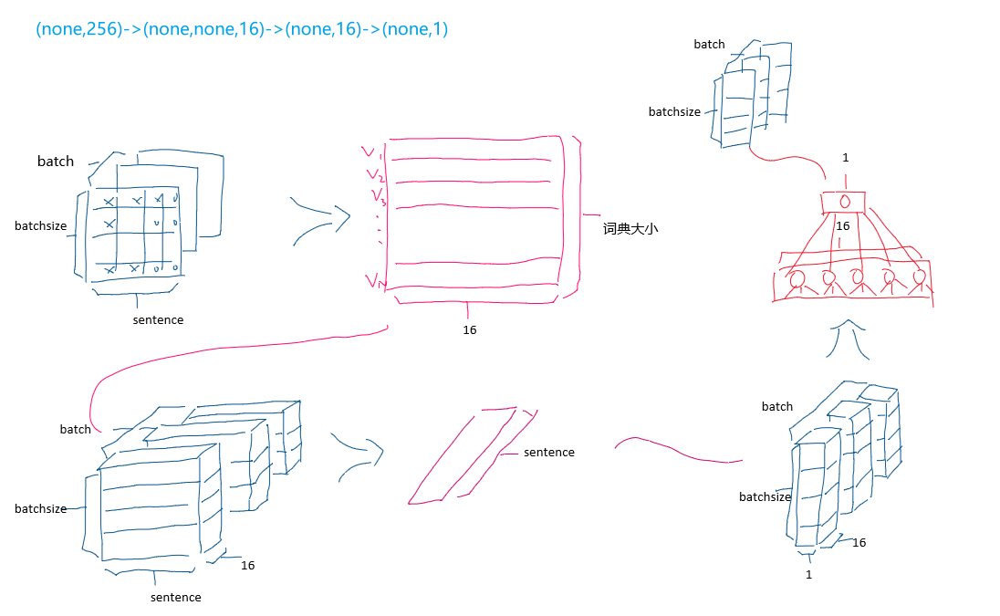
Model: "sequential_1"
_________________________________________________________________
Layer (type)                 Output Shape              Param #   
=================================================================
embedding (Embedding)        (None, None, 16)          160000    
_________________________________________________________________
global_average_pooling1d (Gl (None, 16)                0         
_________________________________________________________________
dense_2 (Dense)              (None, 16)                272       
_________________________________________________________________
dense_3 (Dense)              (None, 1)                 17        
=================================================================
Total params: 160,289
Trainable params: 160,289
Non-trainable params: 0
_________________________________________________________________

9235193169.png
9235193169.png

model.compile(optimizer='adam',
              loss='binary_crossentropy',
              metrics=['accuracy'])
x_val = train_data[:10000]
partial_x_train = train_data[10000:]

y_val = train_labels[:10000]
partial_y_train = train_labels[10000:]
history = model.fit(partial_x_train,
                    partial_y_train,
                    epochs=40,
                    batch_size=512,
                    validation_data=(x_val, y_val),
                    verbose=1)
Train on 15000 samples, validate on 10000 samples
Epoch 1/40
15000/15000 [==============================] - 2s 157us/sample - loss: 0.6917 - accuracy: 0.5409 - val_loss: 0.6893 - val_accuracy: 0.6497
Epoch 2/40
15000/15000 [==============================] - 1s 95us/sample - loss: 0.6843 - accuracy: 0.7176 - val_loss: 0.6789 - val_accuracy: 0.7162
Epoch 3/40
15000/15000 [==============================] - 1s 94us/sample - loss: 0.6698 - accuracy: 0.7300 - val_loss: 0.6614 - val_accuracy: 0.7448
Epoch 4/40
15000/15000 [==============================] - 1s 94us/sample - loss: 0.6463 - accuracy: 0.7591 - val_loss: 0.6353 - val_accuracy: 0.7636
Epoch 5/40
15000/15000 [==============================] - 1s 94us/sample - loss: 0.6136 - accuracy: 0.7847 - val_loss: 0.6019 - val_accuracy: 0.7899
Epoch 6/40
15000/15000 [==============================] - 1s 95us/sample - loss: 0.5736 - accuracy: 0.8143 - val_loss: 0.5633 - val_accuracy: 0.8082
Epoch 7/40
15000/15000 [==============================] - 1s 93us/sample - loss: 0.5301 - accuracy: 0.8335 - val_loss: 0.5227 - val_accuracy: 0.8207
Epoch 8/40
15000/15000 [==============================] - 1s 94us/sample - loss: 0.4857 - accuracy: 0.8509 - val_loss: 0.4839 - val_accuracy: 0.8340
Epoch 9/40
15000/15000 [==============================] - 1s 94us/sample - loss: 0.4442 - accuracy: 0.8620 - val_loss: 0.4494 - val_accuracy: 0.8456
Epoch 10/40
15000/15000 [==============================] - 1s 94us/sample - loss: 0.4070 - accuracy: 0.8723 - val_loss: 0.4194 - val_accuracy: 0.8519
Epoch 11/40
15000/15000 [==============================] - 1s 94us/sample - loss: 0.3750 - accuracy: 0.8808 - val_loss: 0.3944 - val_accuracy: 0.8584
Epoch 12/40
15000/15000 [==============================] - 1s 95us/sample - loss: 0.3473 - accuracy: 0.8897 - val_loss: 0.3740 - val_accuracy: 0.8630
Epoch 13/40
15000/15000 [==============================] - 1s 94us/sample - loss: 0.3240 - accuracy: 0.8946 - val_loss: 0.3573 - val_accuracy: 0.8679
Epoch 14/40
15000/15000 [==============================] - 1s 94us/sample - loss: 0.3035 - accuracy: 0.8991 - val_loss: 0.3434 - val_accuracy: 0.8706
Epoch 15/40
15000/15000 [==============================] - 1s 95us/sample - loss: 0.2857 - accuracy: 0.9041 - val_loss: 0.3325 - val_accuracy: 0.8720
Epoch 16/40
15000/15000 [==============================] - 1s 94us/sample - loss: 0.2699 - accuracy: 0.9094 - val_loss: 0.3227 - val_accuracy: 0.8751
Epoch 17/40
15000/15000 [==============================] - 1s 95us/sample - loss: 0.2559 - accuracy: 0.9133 - val_loss: 0.3159 - val_accuracy: 0.8757
Epoch 18/40
15000/15000 [==============================] - 1s 94us/sample - loss: 0.2433 - accuracy: 0.9179 - val_loss: 0.3080 - val_accuracy: 0.8790
Epoch 19/40
15000/15000 [==============================] - 1s 95us/sample - loss: 0.2313 - accuracy: 0.9223 - val_loss: 0.3029 - val_accuracy: 0.8802
Epoch 20/40
15000/15000 [==============================] - 1s 95us/sample - loss: 0.2208 - accuracy: 0.9253 - val_loss: 0.2983 - val_accuracy: 0.8820
Epoch 21/40
15000/15000 [==============================] - 1s 95us/sample - loss: 0.2108 - accuracy: 0.9289 - val_loss: 0.2944 - val_accuracy: 0.8830
Epoch 22/40
15000/15000 [==============================] - 1s 95us/sample - loss: 0.2020 - accuracy: 0.9322 - val_loss: 0.2914 - val_accuracy: 0.8837
Epoch 23/40
15000/15000 [==============================] - 1s 94us/sample - loss: 0.1931 - accuracy: 0.9363 - val_loss: 0.2890 - val_accuracy: 0.8845
Epoch 24/40
15000/15000 [==============================] - 1s 95us/sample - loss: 0.1852 - accuracy: 0.9397 - val_loss: 0.2884 - val_accuracy: 0.8829
Epoch 25/40
15000/15000 [==============================] - 1s 95us/sample - loss: 0.1791 - accuracy: 0.9421 - val_loss: 0.2861 - val_accuracy: 0.8837
Epoch 26/40
15000/15000 [==============================] - 1s 95us/sample - loss: 0.1709 - accuracy: 0.9466 - val_loss: 0.2857 - val_accuracy: 0.8835
Epoch 27/40
15000/15000 [==============================] - 1s 95us/sample - loss: 0.1643 - accuracy: 0.9495 - val_loss: 0.2844 - val_accuracy: 0.8850
Epoch 28/40
15000/15000 [==============================] - 1s 95us/sample - loss: 0.1579 - accuracy: 0.9523 - val_loss: 0.2839 - val_accuracy: 0.8870
Epoch 29/40
15000/15000 [==============================] - 1s 94us/sample - loss: 0.1518 - accuracy: 0.9546 - val_loss: 0.2847 - val_accuracy: 0.8842
Epoch 30/40
15000/15000 [==============================] - 1s 94us/sample - loss: 0.1471 - accuracy: 0.9557 - val_loss: 0.2845 - val_accuracy: 0.8866
Epoch 31/40
15000/15000 [==============================] - 1s 95us/sample - loss: 0.1407 - accuracy: 0.9578 - val_loss: 0.2852 - val_accuracy: 0.8874
Epoch 32/40
15000/15000 [==============================] - 1s 94us/sample - loss: 0.1361 - accuracy: 0.9600 - val_loss: 0.2866 - val_accuracy: 0.8859
Epoch 33/40
15000/15000 [==============================] - 1s 95us/sample - loss: 0.1312 - accuracy: 0.9617 - val_loss: 0.2874 - val_accuracy: 0.8854
Epoch 34/40
15000/15000 [==============================] - 1s 95us/sample - loss: 0.1261 - accuracy: 0.9640 - val_loss: 0.2895 - val_accuracy: 0.8851
Epoch 35/40
15000/15000 [==============================] - 1s 95us/sample - loss: 0.1218 - accuracy: 0.9661 - val_loss: 0.2905 - val_accuracy: 0.8854
Epoch 36/40
15000/15000 [==============================] - 1s 94us/sample - loss: 0.1175 - accuracy: 0.9678 - val_loss: 0.2924 - val_accuracy: 0.8855
Epoch 37/40
15000/15000 [==============================] - 1s 95us/sample - loss: 0.1132 - accuracy: 0.9695 - val_loss: 0.2946 - val_accuracy: 0.8848
Epoch 38/40
15000/15000 [==============================] - 1s 94us/sample - loss: 0.1093 - accuracy: 0.9705 - val_loss: 0.2968 - val_accuracy: 0.8839
Epoch 39/40
15000/15000 [==============================] - 1s 95us/sample - loss: 0.1056 - accuracy: 0.9720 - val_loss: 0.2998 - val_accuracy: 0.8841
Epoch 40/40
15000/15000 [==============================] - 1s 95us/sample - loss: 0.1023 - accuracy: 0.9733 - val_loss: 0.3016 - val_accuracy: 0.8836
results = model.evaluate(test_data,  test_labels, verbose=2)

print(results)
25000/1 - 2s - loss: 0.3204 - accuracy: 0.8729
[0.3223323440361023, 0.87288]
history_dict = history.history
history_dict.keys()
dict_keys(['loss', 'accuracy', 'val_loss', 'val_accuracy'])
import matplotlib.pyplot as plt

acc = history_dict['accuracy']
val_acc = history_dict['val_accuracy']
loss = history_dict['loss']
val_loss = history_dict['val_loss']

epochs = range(1, len(acc) + 1)

# “bo”代表 "蓝点"
plt.plot(epochs, loss, 'bo', label='Training loss')
# b代表“蓝色实线”
plt.plot(epochs, val_loss, 'b', label='Validation loss')
plt.title('Training and validation loss')
plt.xlabel('Epochs')
plt.ylabel('Loss')
plt.legend()

plt.show()
plt.clf()   # 清除数字

plt.plot(epochs, acc, 'bo', label='Training acc')
plt.plot(epochs, val_acc, 'b', label='Validation acc')
plt.title('Training and validation accuracy')
plt.xlabel('Epochs')
plt.ylabel('Accuracy')
plt.legend()

plt.show()


